Andrew Valentine

Inverse Theory
If we know that \(d = g(m)\), and we are able to measure \(d\), what can we say about \(m\)? Inverse theory is the branch of maths that attempts to address this question. It is particularly relevant to the geosciences, because we often need to study things that we aren’t able to directly observe or measure: we can’t travel back in time to record what the Earth looked like 1 million years ago, or travel deep inside the planet to see exactly what’s down there. Instead, we have to answer these questions as best we can, using only information we can collect at the surface, and at the present day.
I wrote a book chapter that provides an overview of current progress in geophysical inverse theory.1
Contents
- Discrete, linear inverse problems and regularisation
- Continuous linear inverse problems
- Prior sampling
- Optimal Transport
- McMC Sampling
Discrete, linear inverse problems and regularisation
Linear (or linearised) inverse problems are those where the ‘forward model’ \(g\) is known (or assumed) to be linear operator. If we have a finite set of unknowns, we can express them as an \(M\)-dimensional vector \(\mathbf{m}\), and write \(\mathbf{d} = \mathbf{Gm}\), where \(\mathbf{d}\) is an \(N\)-dimensional vector of observations, and \(\mathbf{G}\) is an \(N \times M\) matrix reresenting the linear operator. Usually the data do not constrain all model parameters equally (‘non-uniqueness’), and it is necessary to introduce additional constraints (known as ‘regularisation’) to ensure that a solution can be found. Classically, we use the Gauss-Newton algorithm and obtain a solution:
\[\mathbf{m} = \left[\mathbf{G^TG}+\epsilon^2\mathbf{D}\right]^\mathbf{-1}\mathbf{G^Td}\]where \(\mathbf{D}\) is some regularisation (or damping) matrix, and $\epsilon^2$ is a positive scalar that can be tuned to adjust the strength of regularisation.
Some questions I’ve worked on:
- If your model parameters \(\mathbf{m}\) fall into two or more distinct physical groups (for example, if some describe earth structure, and others describe earthquakes), how should you solve the inverse problem? My first paper explored some different algorithms and highlights the potential for misleading results.2
- Does it matter if your matrix \(\mathbf{G}\) is known to be inaccurate? Various tomographic models (e.g. SEMum2) relied on using physical approximations to construct \(\mathbf{G}\), and it was argued that this had negligible impact on results. I demonstrated that this was not true: over multiple iterations, artefacts can accumulate – which may explain some of the more remarkable features of the resulting models.3
- How do you choose a sensible value for \(\epsilon^2\)? I developed some efficient algorithms to do this based on a hierarchical Bayesian approach.4 A reference implementation of those algorithms is available here.
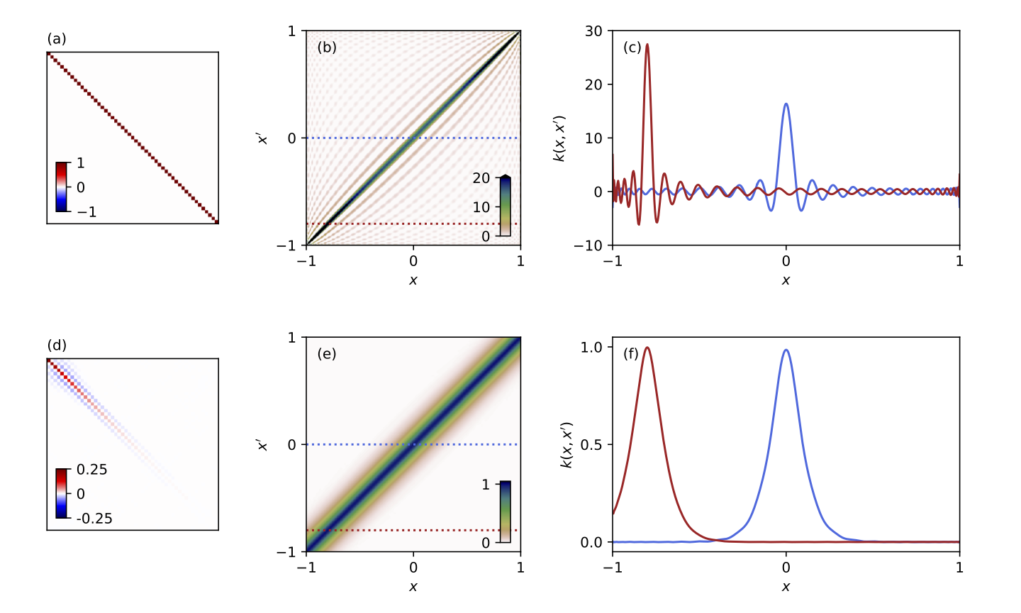
- What is the regularisation actually doing to your results? I showed that this can easily be understood as a covariance function.5
Continuous, linear inverse problems
 Inference for Earth’s radial density structure using a Gaussian process. Only three pieces of information were used: Earth’s mass, moment of inertia, and the mean density of surface rocks.6
In many physically-motivated inverse problems, we want to characterise a continuous function – for example, the velocity of seismic waves at every point within the Earth. One strategy is to discretize the problem by expanding the unknown function in terms of some basis, \(f(x) = \sum_i m_i \phi_i(x)\), and then solving a discrete linear inverse problem for the \(m_i\). However, this can produce misleading results (e.g. spectral leakage). I showed how the model can instead be represented as a Gaussian Process,6 allowing spectral leakage to be avoided.7
Prior Sampling
Prior sampling is an approach to solving inverse problems that leverages machine learning to achieve rapid, computationally-efficient solutions. See this page for more details.
Optimal Transport
McMC sampling
Contents
Back to research overview
References
-
Valentine & Sambridge, in press. Emerging Directions in Geophysical Inversion, To appear as chapter in Data Assimilation and Inverse Problems in Geophysical Sciences, eds. Alik Ismail-Zadeh, Fabio Castelli, Dylan Jones and Sabrina Sanchez. Also available at: arXiv:2110.06017. ↩
-
Valentine & Woodhouse, 2010. Reducing errors in seismic tomography: Combined inversion for sources and structure. doi:10.1111/j.1365-246X.2009.04452.x. ↩
-
Valentine & Trampert, 2016. The impact of approximations and arbitrary choices on geophysical images. doi:10.1093/gji/ggv440. ↩
-
Valentine & Sambridge, 2018. Optimal regularisation for a class of linear inverse problem. doi:10.1093/gji/ggy303. ↩
-
Valentine & Sambridge, 2020. Gaussian process models — II. Lessons for discrete inversion. doi:10.1093/gji/ggz521. ↩
-
Valentine & Sambridge, 2020. Gaussian process models — I. A framework for probabilistic continuous inverse theory. doi:10.1093/gji/ggz520 ↩ ↩2
-
Valentine & Davies, 2020. Global models from sparse data: A robust estimate of Earth’s residual topography spectrum. doi:10.1029/2020GC009240 ↩